\[ \begin{align}\begin{aligned}\newcommand\blank{~\underline{\hspace{1.2cm}}~}\\% Bold symbols (vectors)
\newcommand\bs[1]{\mathbf{#1}}\\% Differential
\newcommand\dd[2][]{\mathrm{d}^{#1}{#2}} % use as \dd, \dd{x}, or \dd[2]{x}\\% Poor man's siunitx
\newcommand\unit[1]{\mathrm{#1}}
\newcommand\num[1]{#1}
\newcommand\qty[2]{#1~\unit{#2}}\\\newcommand\per{/}
\newcommand\squared{{}^2}
\newcommand\cubed{{}^3}
%
% Scale
\newcommand\milli{\unit{m}}
\newcommand\centi{\unit{c}}
\newcommand\kilo{\unit{k}}
\newcommand\mega{\unit{M}}
%
% Percent
\newcommand\percent{\unit{{\kern-4mu}\%}}
%
% Angle
\newcommand\radian{\unit{rad}}
\newcommand\degree{\unit{{\kern-4mu}^\circ}}
%
% Time
\newcommand\second{\unit{s}}
\newcommand\s{\second}
\newcommand\minute{\unit{min}}
\newcommand\hour{\unit{h}}
%
% Distance
\newcommand\meter{\unit{m}}
\newcommand\m{\meter}
\newcommand\inch{\unit{in}}
\newcommand\foot{\unit{ft}}
%
% Force
\newcommand\newton{\unit{N}}
\newcommand\kip{\unit{kip}} % kilopound in "freedom" units - edit made by Sri
%
% Mass
\newcommand\gram{\unit{g}}
\newcommand\g{\gram}
\newcommand\kilogram{\unit{kg}}
\newcommand\kg{\kilogram}
\newcommand\grain{\unit{grain}}
\newcommand\ounce{\unit{oz}}
%
% Temperature
\newcommand\kelvin{\unit{K}}
\newcommand\K{\kelvin}
\newcommand\celsius{\unit{{}^\circ C}}
\newcommand\C{\celsius}
\newcommand\fahrenheit{\unit{{}^\circ F}}
\newcommand\F{\fahrenheit}
%
% Area
\newcommand\sqft{\unit{sq\,\foot}} % square foot
%
% Volume
\newcommand\liter{\unit{L}}
\newcommand\gallon{\unit{gal}}
%
% Frequency
\newcommand\hertz{\unit{Hz}}
\newcommand\rpm{\unit{rpm}}
%
% Voltage
\newcommand\volt{\unit{V}}
\newcommand\V{\volt}
\newcommand\millivolt{\milli\volt}
\newcommand\mV{\milli\volt}
\newcommand\kilovolt{\kilo\volt}
\newcommand\kV{\kilo\volt}
%
% Current
\newcommand\ampere{\unit{A}}
\newcommand\A{\ampere}
\newcommand\milliampereA{\milli\ampere}
\newcommand\mA{\milli\ampere}
\newcommand\kiloampereA{\kilo\ampere}
\newcommand\kA{\kilo\ampere}
%
% Resistance
\newcommand\ohm{\Omega}
\newcommand\milliohm{\milli\ohm}
\newcommand\kiloohm{\kilo\ohm} % correct SI spelling
\newcommand\kilohm{\kilo\ohm} % "American" spelling used in siunitx
\newcommand\megaohm{\mega\ohm} % correct SI spelling
\newcommand\megohm{\mega\ohm} % "American" spelling used in siunitx
%
% Capacitance
\newcommand\farad{\unit{F}}
\newcommand\F{\farad}
\newcommand\microfarad{\micro\farad}
\newcommand\muF{\micro\farad}
%
% Inductance
\newcommand\henry{\unit{H}}
\newcommand\H{\henry}
\newcommand\millihenry{\milli\henry}
\newcommand\mH{\milli\henry}
%
% Power
\newcommand\watt{\unit{W}}
\newcommand\W{\watt}
\newcommand\milliwatt{\milli\watt}
\newcommand\mW{\milli\watt}
\newcommand\kilowatt{\kilo\watt}
\newcommand\kW{\kilo\watt}
%
% Energy
\newcommand\joule{\unit{J}}
\newcommand\J{\joule}
%
% Composite units
%
% Torque
\newcommand\ozin{\unit{\ounce}\,\unit{in}}
\newcommand\newtonmeter{\unit{\newton\,\meter}}
%
% Pressure
\newcommand\psf{\unit{psf}} % pounds per square foot
\newcommand\pcf{\unit{pcf}} % pounds per cubic foot
\newcommand\pascal{\unit{Pa}}
\newcommand\Pa{\pascal}
\newcommand\ksi{\unit{ksi}} % kilopound per square inch
% NOTE: do NOT define \bar -- it is the built-in LaTeX accent used by \bar{x},
% \bar{y} (sample means). Redefining it made those render as the word "bar".
\newcommand\barunit{\unit{bar}}
\end{aligned}\end{align} \]
Nov 16, 2026 | 497 words | 5 min
read
12.2.1. ICA: Good Fit or Bad Fit?
For each dataset below: look at the scatterplot, decide whether linear
regression is a reasonable tool for it, then click Reveal the fit
to check yourself. Don’t peek before you write down an answer!
Dataset A
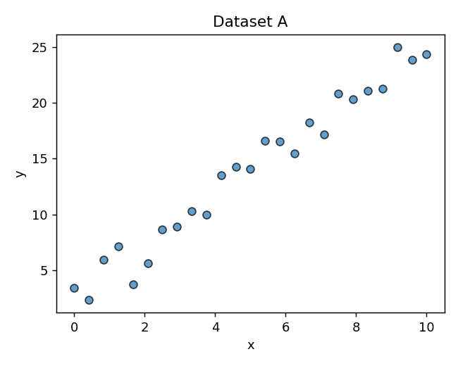
Would you use linear regression here? Why or why not?
Reveal the fit
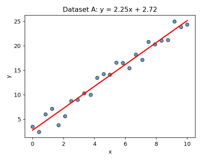
This is what linear regression looks like when it’s a good fit: the
points cluster tightly around a straight line, and the noise looks
about the same size across the whole range of x.
Dataset B
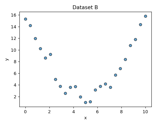
Would you use linear regression here? Why or why not?
Reveal the fit
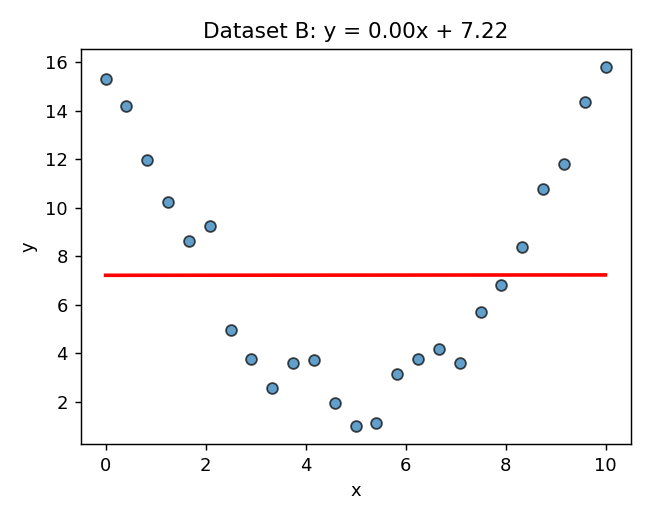
np.polyfit(x, y, 1) will still draw you a line — it doesn’t know any
better — but look how badly it misses the actual (curved) shape of the
data. This relationship is quadratic, not linear. A straight-line model
systematically under- and over-predicts depending on where you are on
the curve.
Dataset C
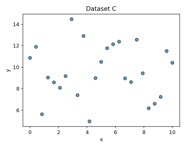
Would you use linear regression here? Why or why not?
Reveal the fit
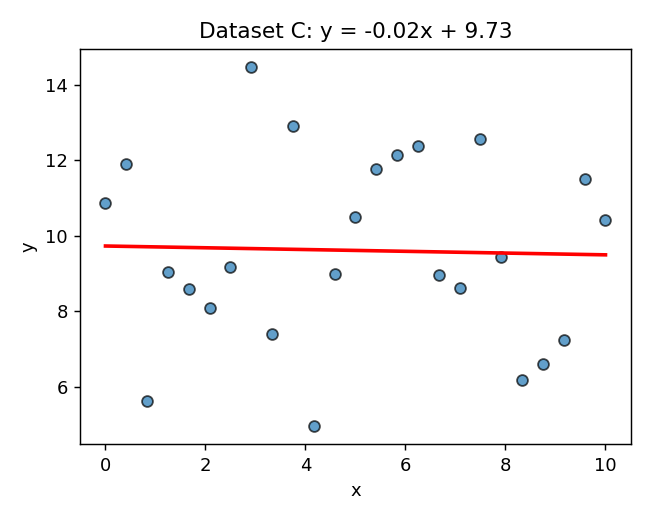
There’s essentially no relationship between x and y here — it’s
just noise around a constant value. polyfit will still return some
slope, but it’s meaningless: don’t mistake “a line got fit” for
“a real relationship exists.”
Dataset D
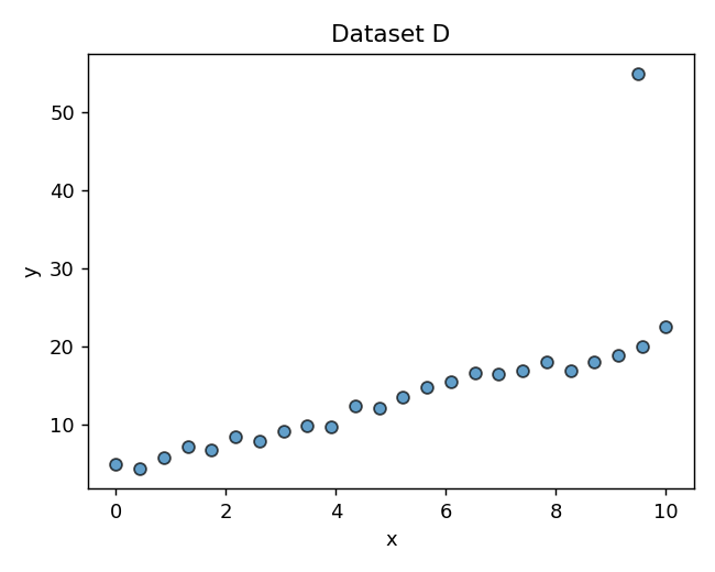
Would you use linear regression here? Why or why not?
Reveal the fit
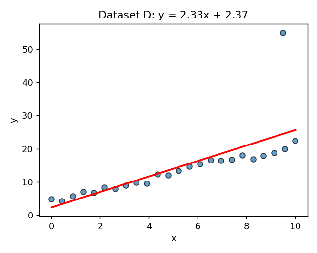
Most of this data is a nice clean linear relationship — except for one
point way out to the upper right. Keep this one in mind for the outlier
question below.
Dataset E
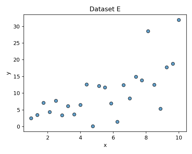
Would you use linear regression here? Why or why not?
Reveal the fit
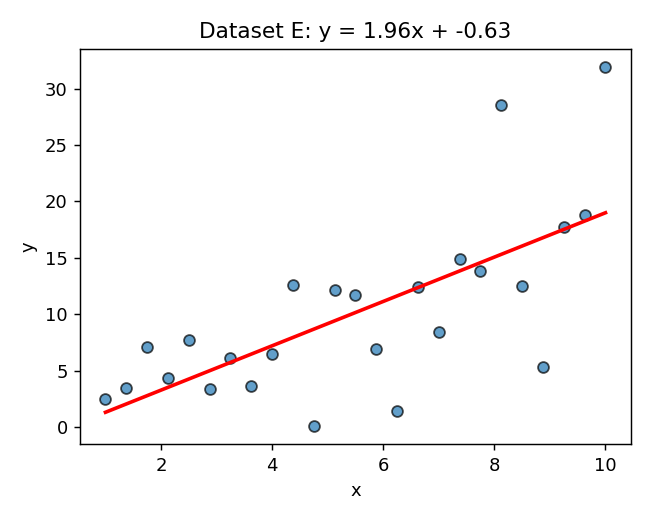
The overall trend does look linear, and the fit isn’t unreasonable —
but notice how the spread of points around the line grows as x
increases (a “fan” or “cone” shape). This is called heteroscedasticity.
It doesn’t mean you can’t use linear regression, but it means your
predictions are much less reliable at large x than at small x, and
some of the standard assumptions behind the model are being violated.
The outlier problem — a closer look at Dataset D
That one extreme point in Dataset D — how much does it actually matter?
Before revealing, make a guess: if we removed it and refit the line,
would the slope change a little or a lot?
Reveal the comparison
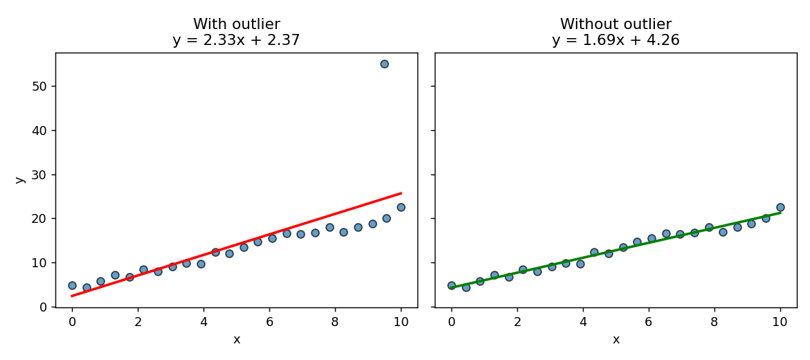
One point moved the slope by more than 35%. That’s the danger of
outliers in a small dataset — a single value can dominate the fit.
Small Group Discussion:
If that point were a data-entry typo, what would you do?
If it were a real, correctly-recorded measurement, would your answer
change? Why?
What might make you more cautious about dropping an outlier
(versus more comfortable doing so)?
Takeaways
np.polyfit() will fit a line to any data you give it — it can’t
tell you whether that line means anything. Look at the scatterplot first.
Good candidates for linear regression: a genuinely straight-line
relationship, with noise that’s roughly the same size across the
whole range of x.
Watch out for: curved relationships (Dataset B), no relationship at
all (Dataset C), spreading/fanning noise (Dataset E), and outliers
(Dataset D) — a single extreme point can swing the slope a lot,
especially in small datasets.
Outliers aren’t automatically “wrong” — figure out why a point is
extreme before deciding to drop it.