
Nov 16, 2026 | 1334 words | 13 min read
5.1.1. PCMs: Probability and Normal Distributions#
These pre-class materials introduce statistical probability and distribution models that engineers use to evaluate reliability and predict outcomes based on data.
In engineering, understanding the likelihood of an event, such as a material failing at a certain stress level, is critical for design and safety.
Relative Probability#
Relative probability determines the likelihood of an event occurring based on collected data. The calculation method depends on whether the data represents a full population or a sample.
When working with a specific dataset (a sample), you can determine the relative probability by comparing the number of times an event occurs to the total number of trials. Engineers often extract these frequency values directly from the bin counts of a histogram.
Example Calculations#
Example 1: Drone Flights#
If a histogram shows that an agricultural drone completed 50 total test flights (total trials), and 15 of those flights lasted longer than 20 minutes (event occurrences), the relative probability of a flight lasting longer than 20 minutes is calculated as:
Example 2: Yellow Skittles#

Fig. 5.1 A red, rectangular wrapper for a Share Size bag of Original Skittles. Image source: Mars Wrigley Confectionery.#
As seen in Fig. 5.1, a bag of Skittles includes five colors. You would likely expect to have about 20% yellow Skittles in every bag. As an industrial engineer at the factory, you must ensure the bag-filling machinery is working properly.
You sample 150 bags of Skittles, count the number of yellow Skittles in each bag, convert the counts to percentages, and create the following histogram:
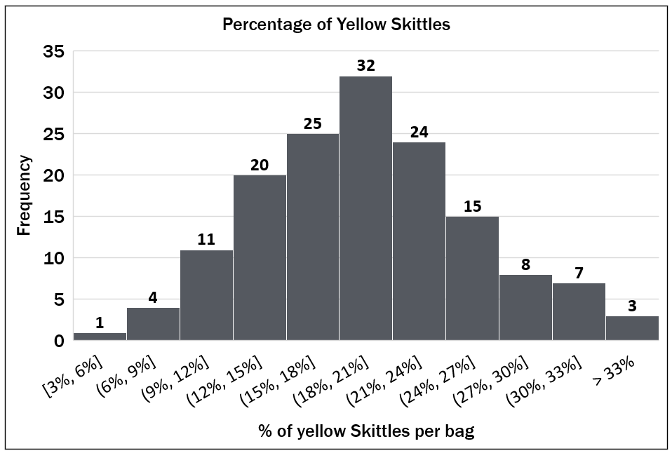
Fig. 5.2 A histogram showing percentage of yellow skittle values grouped into bins along the x-axis, with frequency shown on the y-axis.#
To find the probability, identify the total number of bags containing more than 27% yellow Skittles and divide by the total number of bags sampled.
Locate the bins on the x-axis representing greater than 27%. These are the (27%, 30%], (30%, 33%], and > 33% bins.
Sum the frequencies (y-axis values) of these three bins: 8 + 7 + 3 = 18 bags.
Divide this number of event occurrences (18) by the total number of trials (150 bags).
Check for Understanding
Using Fig. 5.2, what is the relative probability of a random bag from the sample containing between 15% and 24% yellow Skittles?
Show Answer
Correct Answer: 54%.
The bins for 15-24% have frequencies of 25, 32, and 24. Summing these gives 81 event occurrences. There are 150 total trials. \(81 \div 150 = 0.54\)
Normal Distributions#
A normal distribution, often called a bell curve, is a specific way data can be distributed. The probability of an event is represented by a specific portion of the area under this curve.
A perfectly normal distribution has the following properties:
The mean, median, and mode are all equal.
The curve is perfectly symmetric at the center.
The total area under the curve is exactly 1 (or 100%).
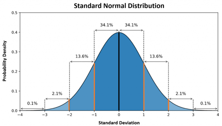
Fig. 5.3 A standard normal distribution curve demonstrating the 68-95-99.7% rule. The percentages represent the probability density within each standard deviation from the mean.#
Check for Understanding
An engineer is analyzing a dataset of drone flight times that perfectly follows a normal distribution. Which of the following statements about the data is true?
A. The mean, median, and mode flight times are all equal.
B. The total area under the distribution curve depends on the number of trials.
C. To calculate a z-score for a flight time, the engineer only needs the median and standard deviation.
D. Exactly 68% of the values are to the left of the center.
Show Answer
Correct Answer: A
The total area is always exactly 1 (100%), regardless of the number of trials.
You also need the specific flight time (the data point) and the mean to calculate a z-score.
The curve is perfectly symmetric, so exactly 50% of values are to the left. 68% refers to the data within one standard deviation from the mean.
Z-Scores#
A z-score measures the distance of a specific data point from the dataset’s mean, expressed in the number of standard deviations. If a dataset is normally distributed, engineers use z-scores to calculate the exact probability of an event occurring without needing to count individual bins on a histogram.
A z-score can be calculated from any data set using the expression:
Where:
\(x\) = data point
\(\mu\) = mean
\(\sigma\) = standard deviation
Information
Z-scores can be efficiently calculated across an entire dataset using the expression above and cell references in Excel.
Using Z-Tables#
Z-tables help find the probability associated with a specific calculated z-score. Standard z-tables only display the area to the left of the curve. You may have to adjust your final calculation depending on the probability you are trying to find.
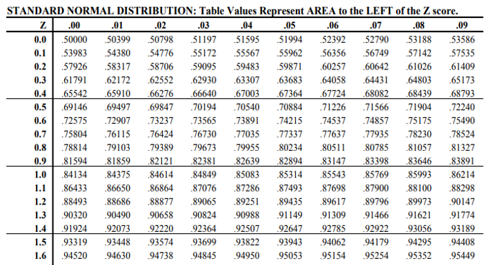
Fig. 5.4 A standard normal distribution z-table used to find the probability, representing the area to the left, of a specific z-score.#
Example: Yellow Skittles#
Imagine you calculate the exact statistics of your 150 Skittles bags. You find the mean (\(\mu\)) is 20% yellow Skittles, with a standard deviation (\(\sigma\)) of 6%. You want to find the exact probability of randomly selecting a bag with more than 27% yellow Skittles (\(x\)).
First, calculate the z-score to find how many standard deviations 27% is from the mean.
From the z-table in Fig. 5.4, the area to the left of a z-score of \(1.16\) is \(0.87698\). That means that there is an 87.698% probability that a random bag contains 27% or fewer yellow Skittles.
However, you want the probability of randomly selecting a bag with more than 27% yellow Skittles, so you will subtract your value from 1.
Check for Understanding
An engineer is evaluating a new composite material and needs to find the probability of the tensile strength being 72 psi or greater. Using a standard z-table, they find the value corresponding to their calculated z-score is 0.3669. What is the correct next step to find the final probability?
A. Multiply 0.3669 by the standard deviation of the tensile strength.
B. Use 0.3669 as the final probability, because the z-table directly provides the
probability to the right.
C. Subtract 0.3669 from 1, because the standard z-table only provides the probability to
the left of the z-score.
D. Subtract the z-score from 0.3669.
Show Answer
Correct Answer: C
You do not multiply the table probability value by the standard deviation.
Standard z-tables provide the probability to the left of the curve, not the right.
Subtracting the z-score from the probability value is not a valid statistical operation.
Finding Probabilities Using Excel Built-In Functions#
While standard paper Z-tables are valuable for learning the hand-calculated mechanics of standardization, they require you to round your Z-scores to two decimal places which can introduce small precision errors. In professional engineering practice, you will use Excel’s built-in, high-precision statistical functions to calculate exact cumulative probabilities directly from raw or standardized data.
The Two Core Normal Distribution Functions#
Excel provides two primary functions for evaluating normal distributions:
=NORM.DIST()(The Raw Value Method): Used when you want to calculate a probability directly from a raw engineering measurement (x), its sample mean (\(\mu\)), and standard deviation (\(\sigma\)). Excel handles the z-score (standardization) calculation internally.=NORM.S.DIST()(The Standardized Method): The “S” in this function stands for Standard. This function expects a pre-calculated, standardized Z-score. It acts as a digital, high-precision version of your paper Z-table.
To calculate a cumulative probability, use the formulas structured in the table below:
Calculation Goal |
Excel Function Syntax |
Arguments Defined |
Probability Visual |
|---|---|---|---|
Area to the LEFT |
|
|
Left-Tail Area |
Standardized Area to the LEFT |
|
|
Left-Tail Area |
Area to the RIGHT |
|
|
Right-Tail Area |
Standardized Area to the RIGHT |
|
|
Right-Tail Area |
The Critical “Cumulative” Trap (TRUE vs. FALSE)
The final argument in both functions is the cumulative logical switch:
Always use
TRUE: Setting this parameter toTRUEtells Excel to calculate the cumulative area under the curve from negative infinity up to your value (the cumulative distribution function, or CDF). This is the only setting that returns a probability.Never use
FALSE: If you accidentally enterFALSE, Excel will calculate the height of the curve at that exact single point (the probability density function, or PDF). In continuous distributions, the probability of a single exact point is mathematically zero, so this height metric is useless for reliability calculations.