
Nov 16, 2026 | 573 words | 6 min read
5.2.1. ICA: Semiconductor Quality Control#
In microelectronics fabrication, the gate oxide layer acts as the physical barrier separating a transistor’s gate from its conductive channel.
The Safety Threshold: To ensure high-frequency performance and prevent quantum tunneling leakage, a semiconductor design team specifies a minimum gate oxide thickness of \(90.0 \text{nm}\). Any wafer with a gate oxide falling below \(90.0 \text{nm}\) is a catastrophic structural failure, causing device short-circuits and rendering the processor useless.
The Quality Investigation: A process control team is evaluating two deposition machines (Tool 1 and Tool 2) that grow this microscopic oxide layer. To gather statistical process data, the engineers grew gate oxides on trial silicon wafers using both tools and recorded their final thickness measurements in nanometers.
The Problem: While both tools appear to produce the same average thickness of \(100.0 \text{nm}\), Tool 2 suffered from an unstable gas flow drift during deposition. You must use Excel statistical and charting tools to evaluate which machine is truly safe for production.
Required Files#
Download the activity template.
Instructions#
Download the provided Excel spreadsheet template and complete the following tasks.
Part A: Summary Statistics and High-Precision Shape Diagnosis#
Before calculating failure risks or modeling the process, verify that your measurements are approximately normally distributed (symmetric, bell-shaped).
Provide a numerical snapshot of both tools. Use Excel’s built-in functions to calculate the required summary statistics. Format these values in Table 1: Baseline Parameter, including units.
For a dataset to be modeled using a standard normal distribution, both its skewness and kurtosis must fall within the stable range of \(-2.0000\) to \(2.0000\). Calculate the following metrics in Table 2: Process Distribution Shape using Excel’s built-in functions for both tools. Leave each value with 4 decimal places.
Skewness:
=SKEW()Kurtosis:
=KURT()
Part B: Creating and Formatting Technical Histograms#
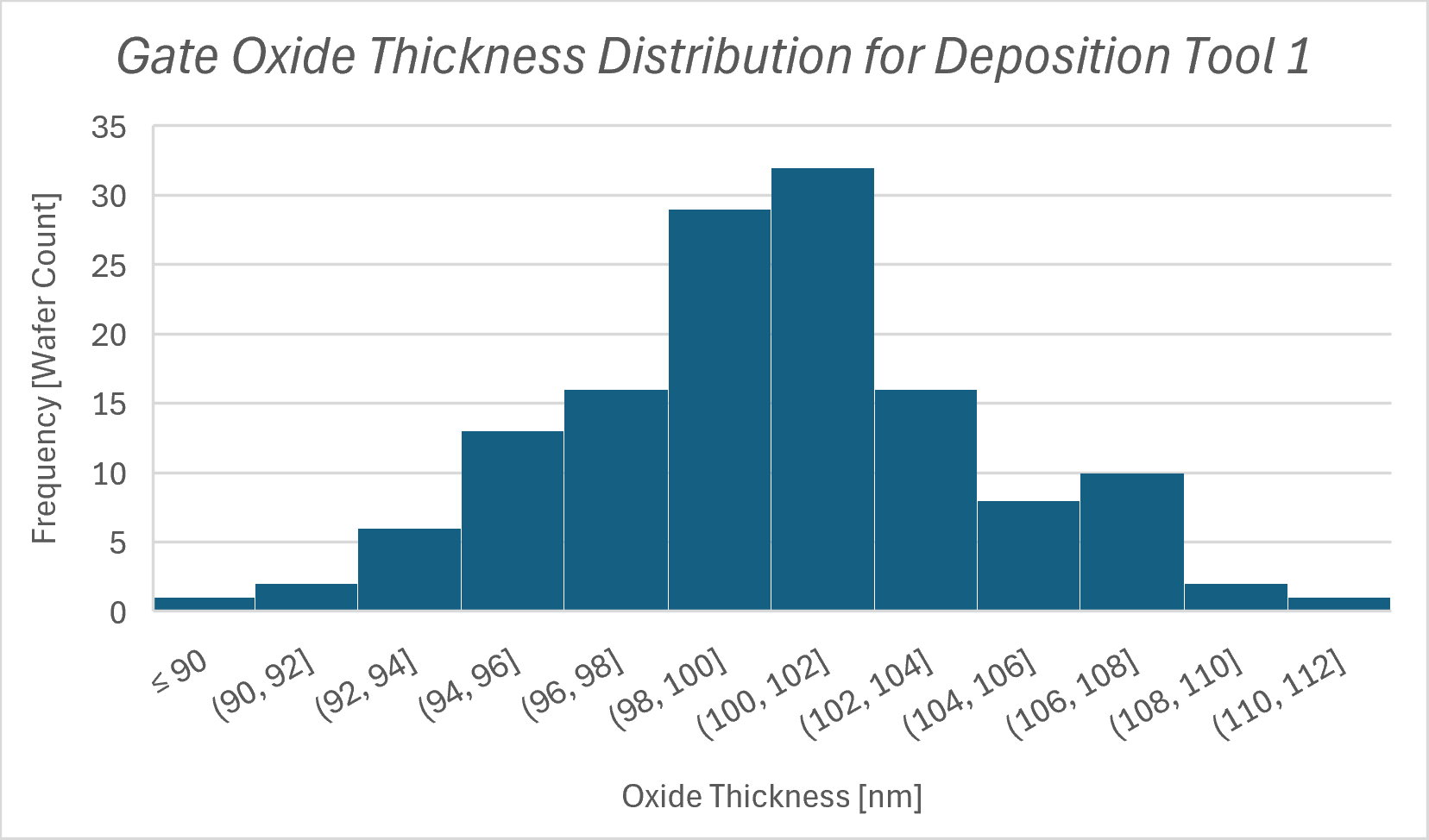
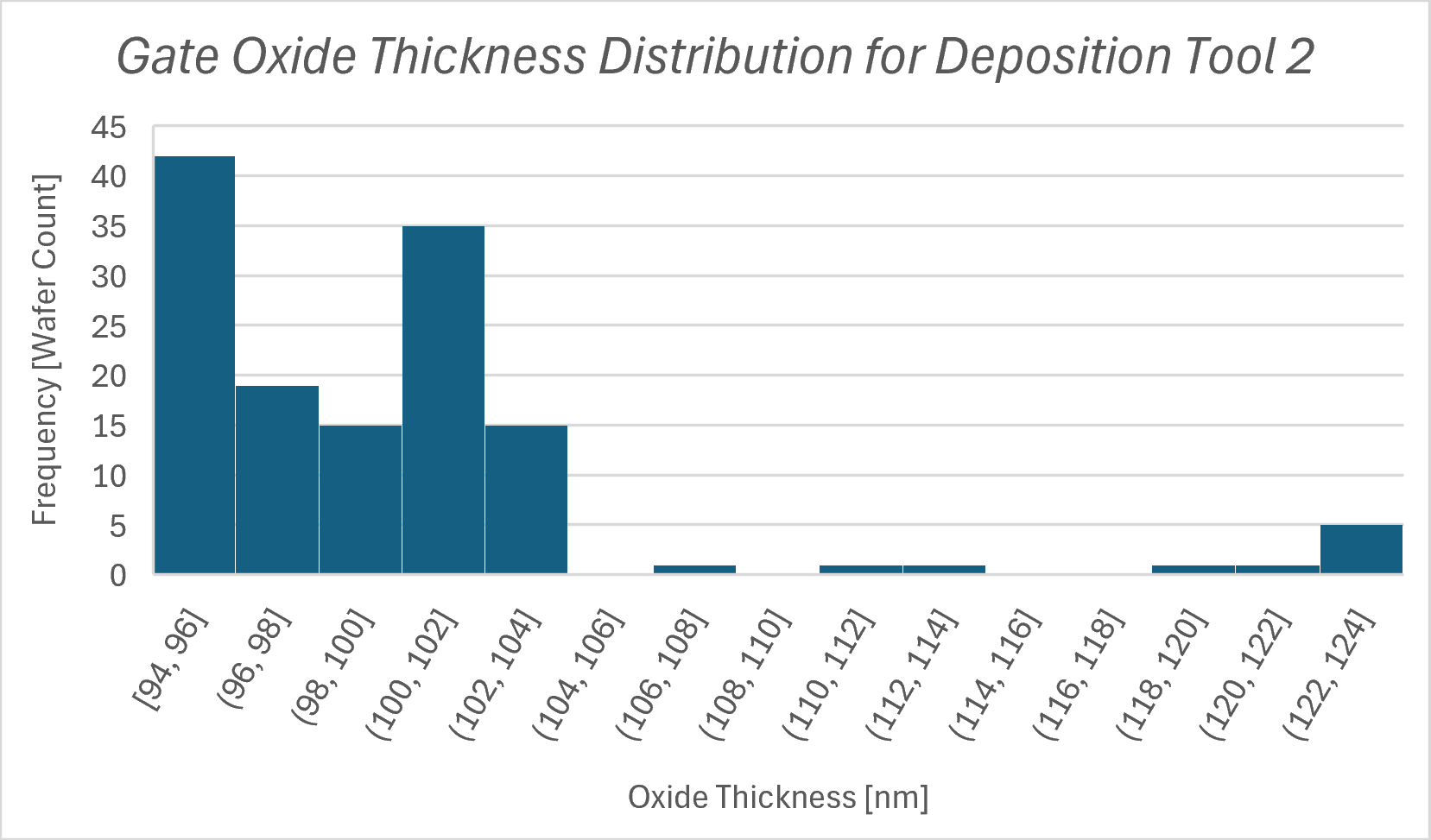
You will now construct two professional histograms to visually analyze how the raw measurements are spread across the deposition intervals.
Formatting Constraints for the Histogram
Bin Width: manually override Excel defaults to use a width of 2.0 nm.
Underflow Bin: set an underflow bin at 90.0 nm. This isolates all wafers that fail the safety requirement into a single bar on the far left.
Chart Title and Axis Labels: use descriptive labels that are appropriate for technical presentation.
Part C: Relative vs. Theoretical Probability Calculations#
You will now program Excel to calculate both the relative failure rate (counting actual occurrences) and the theoretical failure rate (using continuous normal curves) to compare their precision.
In Table 3: Relative Probability Calculations, calculate the Failing Wafer Count using the
=COUNTIF()function to count how many wafers in each of your datasets failed to meet the safety limit.Cross-reference this number with your histograms from Part B. The first bar, the underflow bin, should have the same count.
Calculate the relative probability of failure by dividing your count of failing specimens by the total number of trials. Use cell referencing. Format the cell as a percentage with two decimal places.
In Table 4: Theoretical Probability Calculations, enter the algebraic formula to calculate the z-score for both datasets (standardize your safety limit of \(x = 90 \text{nm}\)). Use cell referencing and format the cell with two decimal places.
Download and open
Z-table. Locate the cumulative left-tail area for both z-scores. Enter both values into “Theoretical Failure Prob (Z-Table)” and format the cells as a percentage with two decimal places.Use
=NORM.S.DIST()and=NORM.DIST()to calculate the remaining probabilities in the table. Use cell references and format the cells as a percentage with two decimal places. Verify that these match your manual lookup for both Tool 1 and Tool 2.